COMSOL LiveLink for MATLAB

COMSOL LiveLink for MATLAB 功能允许用户将 COMSOL Multiphysics 与 MATLAB 脚本环境联系起来，可以实现：

通过脚本设置模型
在模型设置中使用 MATLAB 函数
在 COMSOL Desktop 和 MATLAB 之间进行交互式建模
通过 MATLAB 控制语句调节程序流程
在 MATLAB 中分析结果
创建定制模型接口
······

启动

Windows：双击 COMSOL with MATLAB 图标，启动 COMSOL Multiphysics with MATLAB

MATLAB 的桌面环境将与 COMSOL Multiphysics Server 同时打开，后者以命令窗口的形式显示在背景中
Mac OS X：前往 Applications > COMSOL > COMSOL with MATLAB
Linux：在 COMSOL 安装目录的 bin 文件夹中打开一个终端提示窗口，执行 comsol 命令：comsol mphserver matlab

使用

COMSOL LiveLink for MATLAB 是使用 MATLAB 命令来构建模型，即使用直接操作的是 COMSOL 模型对象，而不是 COMSOL Desktop。

一般有两种使用方法：

在 COMSOL Desktop 的图形化用户界面中完成建模，然后将模型另存为 M 文件，通过修改该文件来满足计算需求

可设置全局变量，并封装为函数，在 MATLAB 中进行调用

一定要在 COMSOL Desktop 中压缩历史记录，以删除建模过程中的无效操作
直接编写 MATLAB 脚本进行建模、计算、分析

学习曲线较高，不建议采用这种方法

API 命令

这里仅展示部分常用 MATLAB 中的 API 命令

mphdoc ：打开 COMSOL 帮助文档（缺省值）

mphdoc(model) ：打开节点模型的帮助文档

mphdoc(model.geom,'WorkPlane') ：打开几何特征 WorkPlane 的帮助文档
mphlaunch ：将正在运行的模型从 MATLAB 提示窗口连接到 COMSOL Desktop
mphgeom(model) ：在 MATLAB 图像窗口中显示当前对象的几何
mphmesh(model) ：在 MATLAB 图像窗口中显示当前对象的网格
ModelUtil.showProgress(true) ：显示求解和网格运算的进度条
mphplot(model,'pg','rangenum',1) ：在 MATLAB 图形中显示包含颜色条的绘图组

rangenum 对应于绘图组 pg 中的绘图类型序号
mphsave(model,'<path>\busbar') ：将模型保存到 <path> 路径下的 busbar 文件中，默认的保存格式为 COMSOL 二进制格式，扩展名为 mph

mphsave(model,'<path>\busbar.m') ：将模型保存成 M 文件

示例

采用《相场损伤模型》中的物理模型，即 \[ \begin{cases} d-l^2\Delta d=0&~\mathrm{in}~V\\[5pt] \nabla d\cdot\boldsymbol{n}=0&~\mathrm{on}~\partial V\\[5pt] d(\boldsymbol{x})=1&~\mathrm{on}~\Gamma \end{cases} \] 对于边长为 2 的正方形（二维）求解域进行计算。

在 COMSOL 中将特征长度参数 \(l\) 、裂纹边的最大单元大小 \(l_e\) 设为全局变量，并在派生值中定义能量耗散函数 \[ \Gamma_l(d)=\frac{1}{2l}\int_{V}\big(d^2+l^2\nabla d\cdot\nabla d\big)\mathrm{d}v \] 完成建模等设置后，将模型另存为 M 文件，并进一步将其修改为函数 PFD_PDE(L,EL) ，代码如下：

% 输入
% L  : 特征尺度参数, 如 0.25
% EL : 裂纹处最大单元尺寸, 如 0.05
function [GAMMA, MODEL] = PFD_PDE(L,EL)

% 导入COMSOL库
import com.comsol.model.*
import com.comsol.model.util.*

% 创建模型
model = ModelUtil.create('Model');

% 指定模型的路径, 名称, 坐标系
model.modelPath(pwd);% 使用当前路径
model.label('PDE_phase_field_damage_2D_TEST.mph');
model.baseSystem('none');

% 设置全局参数'L', 'EL'
model.param.set('L', num2str(L), 'Characteristic length');
model.param.set('EL',num2str(EL),'Crack unit size');

% 创建组件'geom1'
model.component.create('comp1', true);

% 定义组件中几何体的个数
model.component('comp1').geom.create('geom1', 2);

% 定义组件的网格'mesh1'
model.component('comp1').mesh.create('mesh1');

% 创建几何体中的正方形'sq1'
model.component('comp1').geom('geom1').create('sq1', 'Square');
model.component('comp1').geom('geom1').feature('sq1').set('pos', [0 0]);
model.component('comp1').geom('geom1').feature('sq1').set('base', 'center');
model.component('comp1').geom('geom1').feature('sq1').set('size', 2);

% 创建几何体中的线段'ls1'
model.component('comp1').geom('geom1').create('ls1', 'LineSegment');
model.component('comp1').geom('geom1').feature('ls1').set('specify1', 'coord');
model.component('comp1').geom('geom1').feature('ls1').set('coord1', [-1 0]);
model.component('comp1').geom('geom1').feature('ls1').set('specify2', 'coord');
model.component('comp1').geom('geom1').run;

% 对组件添加物理场, 即系数型偏微分方程'c'
model.component('comp1').physics.create('c', 'CoefficientFormPDE', 'geom1');

% 设置物理场的名称'd', 变量'd'
model.component('comp1').physics('c').field('dimensionless').field('d');
model.component('comp1').physics('c').field('dimensionless').component({'d'});

% 设置物理场中的狄氏条件, 即用狄氏条件描述裂纹
model.component('comp1').physics('c').create('dir1', 'DirichletBoundary', 1);
model.component('comp1').physics('c').feature('dir1').selection.set(4);

% 设置裂纹边处的网格
model.component('comp1').mesh('mesh1').create('edg1', 'Edge');
model.component('comp1').mesh('mesh1').feature('edg1').selection.set(4);
model.component('comp1').mesh('mesh1').feature('edg1').create('size1', 'Size');

% 网格'mesh1'采用自由三角形划分
model.component('comp1').mesh('mesh1').create('ftri1', 'FreeTri');

% 设置可视化区域范围
model.component('comp1').view('view1').axis.set('xmin', -1.7);
model.component('comp1').view('view1').axis.set('xmax', 1.7);
model.component('comp1').view('view1').axis.set('ymin', -1.2);
model.component('comp1').view('view1').axis.set('ymax', 1.2);

% 设置系数型偏微分方程中的参数
model.component('comp1').physics('c').prop('Units').set('CustomSourceTermUnit', 1);
model.component('comp1').physics('c').feature('cfeq1').set('c', {'L^2' '0' '0' 'L^2'});
model.component('comp1').physics('c').feature('cfeq1').set('a', 1);
model.component('comp1').physics('c').feature('cfeq1').set('f', 0);
model.component('comp1').physics('c').feature('cfeq1').set('da', 0);

% 设置裂纹处狄氏条件的值, 即令该处d=1
model.component('comp1').physics('c').feature('dir1').set('r', 1);

% 网格剖分: 非裂纹处, 最大单位大小为'3*EL', 最大单元增长率为1.1
model.component('comp1').mesh('mesh1').feature('size').set('custom', 'on');
model.component('comp1').mesh('mesh1').feature('size').set('hmax', '3*EL');
model.component('comp1').mesh('mesh1').feature('size').set('hgrad', 1.1);

% 网格剖分: 裂纹处, 并将最大单位大小设置为'EL' (需要激活设置, 即'hmaxactive')
model.component('comp1').mesh('mesh1').feature('edg1').feature('size1').set('hauto', 3);
model.component('comp1').mesh('mesh1').feature('edg1').feature('size1').set('custom', 'on');
model.component('comp1').mesh('mesh1').feature('edg1').feature('size1').set('hmax', 'EL');
model.component('comp1').mesh('mesh1').feature('edg1').feature('size1').set('hmaxactive', true);

% 生成网格'mesh1'
model.component('comp1').mesh('mesh1').run;

% 创建稳态分析'std1'
model.study.create('std1');
model.study('std1').create('stat', 'Stationary');

% 配置求解器, 采用默认参数
model.sol.create('sol1');
model.sol('sol1').study('std1');
model.sol('sol1').attach('std1');
model.sol('sol1').create('st1', 'StudyStep');
model.sol('sol1').create('v1', 'Variables');
model.sol('sol1').create('s1', 'Stationary');
model.sol('sol1').feature('s1').create('fc1', 'FullyCoupled');
model.sol('sol1').feature('s1').feature.remove('fcDef');

% 创建派生值'int1', 即表面积分Gamma
model.result.numerical.create('int1', 'IntSurface');
model.result.numerical('int1').selection.all;
model.result.numerical('int1').set('probetag', 'none');

% 创建二维绘图组'pg1', 表面数据'surf1'
model.result.create('pg1', 'PlotGroup2D');
model.result('pg1').create('surf1', 'Surface');

% 关联研究与求解器
model.sol('sol1').attach('std1');

% 运行模型, 得到计算结果
model.sol('sol1').runAll;

% 设置表面积分Gamma
model.result.numerical('int1').label('int_Gamma');
model.result.numerical('int1').set('expr', {'(d^2+L^2*(dx^2+dy^2))/2/L'});
model.result.numerical('int1').set('descr', {'Gamma'});

% 设置表面绘制
model.result('pg1').feature('surf1').set('resolution', 'normal');

% 创建表格, 用于存储表面积分Gamma
model.result.table.create('tbl1', 'Table');
model.result.table('tbl1').comments('int_Gamma {int1} ((d^2+L^2*(dx^2+dy^2))/2/L)');
model.result.numerical('int1').set('table', 'tbl1');
model.result.numerical('int1').setResult;

% 输出
temp = mphtable(model,'tbl1');
GAMMA = temp.data;% 能量耗散函数
MODEL = model;% 模型对象

end

在函数 PFD_PDE(L,EL) 的基础上，可以做出更多的扩展计算。

计算绘图

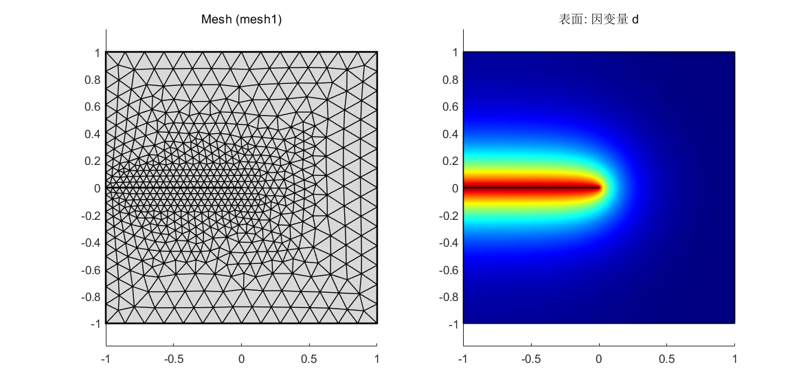
给定 L 和 EL 后可调用函数 PFD_PDE(L,EL) ，计算得到模型对象的句柄 MODEL 。进一步利用 API 命令 mphmesh 和 mphplot 得到网格和相场云图，代码如下：

clc;clear;close;

set(0,'units','centimeters')
cm_ss=get(0,'screensize');
W=cm_ss(3);H=cm_ss(4);% 屏幕尺寸
fw=25;fh=12;% 图片尺寸

[gamma, model] = PFD_PDE(0.25,0.05);

figure(1);
set(gcf,'units','normalized','position',[(W-fw)/2/W,(H-fh)/2/H,fw/W,fh/H]);
subplot(1,2,1);mphmesh(model);
subplot(1,2,2);mphplot(model,'pg1');

上述代码运行结果如下：

封装调用

给定 EL 并遍历 L ，调用函数 PFD_PDE(L,EL) ，可得特征长度参数 \(l\) 与能量耗散函数 \(\Gamma_l\) 的数值映射表，代码如下：

clc;clear;close;

num=20;
L=linspace(0.05,1,num);
gamma=zeros(1,num);
for i=1:num
    [gamma(i),~] = PFD_PDE(L(i),0.05);
end

pt=15;
plot(L,gamma,'linewidth',1.5,'LineStyle','-','Color',[0,0,0]);
box on;grid on;xlim([0,1.05]);
set(gca,'fontsize',pt,'ticklabelinterpreter','latex');
xlabel('Length  $l$','FontSize',pt,'Interpreter','latex');
ylabel('Energy  $\Gamma_l$','FontSize',pt,'Interpreter','latex');

上述代码运行结果如下：

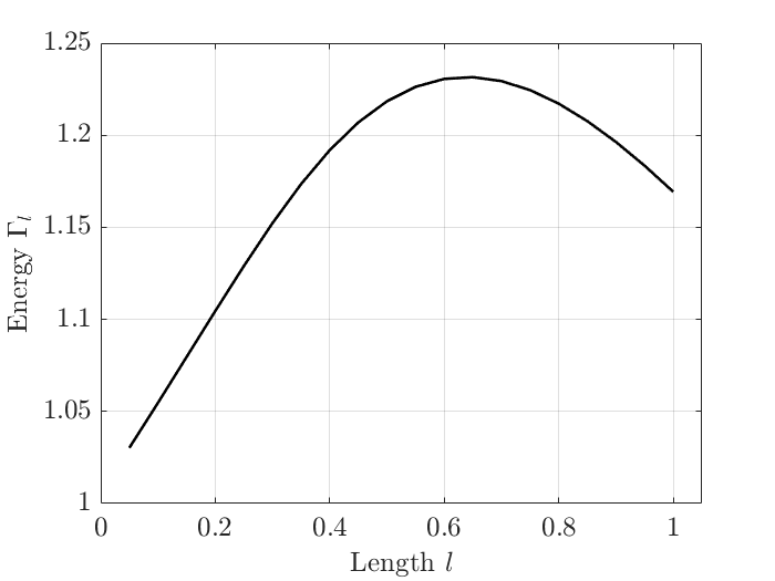
显然函数 \(\Gamma_l(l)\) 在 0.6 附近存在一个局部极大值，于是可调用 MATLAB 中的粒子群优化函数进行求解，代码如下：

优化函数 fmincon 需要目标函数的导数信息（给定解析导函数或求数值导数），而这种基于有限元计算得到数值，其连续性不佳，导致函数 fmincon 无法得到较好的优化结果

粒子群优化函数 particleswarm 则不需要目标函数的导数信息，以随机地形式寻找全局最优

clc;clear;close;

fun = @(x) -PFD_PDE(x,0.05);

options = optimoptions('particleswarm','SwarmSize',5,...
                       'FunctionTolerance',1e-2,'MaxIterations',50);
Lmin = particleswarm(fun,1,0.4,0.8,options);% PFD_PDE(0.6396,0.05)=1.2316

上述代码运行结果得到：Lmin = 0.6396

止于至善